The Wonderful Relationship Between Integration And Euler’s Quantity

We use integration to measure lengths, areas, or volumes. It is a geometrical interpretation, however we need to study an analytical interpretation that leads us to Integration reverses differentiation. Therefore allow us to begin with differentiation.

Weierstraß Definition of Derivatives

##f## is differentiable at ##x## if there’s a linear map ##D_{x}f##, such that
start{equation*}
underbrace{D_{x}(f)}_{textual content{By-product}}cdot underbrace{v}_{textual content{Course}}=left(left. dfrac{df(t)}{dt}proper|_{t=x}proper)cdot v=underbrace{f(x+v)}_{textual content{location plus change}}-underbrace{f(x)}_{textual content{location}}-underbrace{o(v)}_{textual content{error}}
finish{equation*}
the place the error ##o(v)## will increase slower than linear (cp. Landau image). The spinoff may be the Jacobi-matrix, a gradient, or just a slope. It’s at all times an array of numbers. If we converse of derivatives as features, then we imply ##f’, : ,xlongmapsto D_{x}f.## Integration is the issue to compute ##f## from ##f’## or ##f## from
$$
dfrac{f(x+v)-f(x)}+o(1)
$$
The quotient on this expression is linear in ##f## so
$$
D_x(alpha f+beta g)=alpha D_x(f)+beta D_x(g)
$$
If we add the Leibniz rule
$$
D_x(fcdot g)=D_{x}(f)cdot g(x) + f(x)cdot D_{x}(g)
$$
and the chain rule
$$
D_x(fcirc g)=D_{g(x)}(f)circ g cdot D_x(g)
$$
then we’ve got the primary properties of differentiation.

Integration Guidelines

The answer ##f(x)## given ##D_x(f)## is written
$$
f(x)=int D_x(f),dx=int f'(x),dx
$$
which can be linear
$$
int left(alpha f'(x)+beta g'(x)proper),dx = alpha int f'(x),dx +beta int g'(x),dx
$$
and obeys the Leibniz rule which we name integration by components
$$
f(x)g(x)=int D_x(fcdot g),dx=int f'(x)g(x),dx + int f(x)g'(x),dx
$$
and the chain rule results in the substitution rule of integration
start{align*}
f(g(x))=int f'(g(x))dg(x)&=int left.dfrac{df(y)}{dy}proper|_{y=g(x)}dfrac{dg(x)}{dx}dx=int f'(g(x))g'(x)dx
finish{align*}

Differentiation is simple, Integration is troublesome

As a way to differentiate, we have to compute
$$
D_x(f)=lim_{vto 0}left(dfrac{f(x+v)-f(x)}+o(1)proper)=lim_{vto 0}dfrac{f(x+v)-f(x)}
$$
which is a exactly outlined process. Nonetheless, if we need to combine, we’re given a perform ##f## and must discover a perform ##F## such that
$$
f(x)=lim_{vto 0}dfrac{F(x+v)-F(x)}.
$$
The restrict as a computation process isn’t helpful since we have no idea ##F.## Actually, we’ve got to contemplate the pool of all attainable features ##F,## compute the restrict, and examine whether or not it matches the given perform ##f.## And the pool of all attainable features is giant, very giant. The primary integrals are subsequently discovered by the alternative technique: differentiate a identified perform ##F,## compute ##f=D_x(F),## and checklist
$$
F=int D_x(F),dx=int f(x),dx.
$$
as an integral formulation. Positive, there are numerical strategies to compute an integral, nonetheless, this doesn’t result in a closed type with identified features. An enormous and essential class of features is polynomials. So we begin with ##F(x)=x^n.##
start{align*}
D_x(x^n)&=lim_{vto 0}dfrac{(x+v)^n-x^n}=lim_{vto 0}dfrac{binom n 1 x^{n-1}v+binom n 2 x^{n-2}v^2+ldots}=nx^{n-1}
finish{align*}
and get
$$
x^n = int nx^{n-1},dx quadtext{or} quad int x^r,dx = dfrac{1}{r+1}x^{r+1}
$$
and specifically ##int 0,dx = c, , ,int 1,dx = x.## The formulation is even legitimate for any actual quantity ##rneq -1.## However what’s
$$
int dfrac{1}{x},dxtext{ ?}
$$

Euler’s Quantity and the ##mathbf{e}-##Perform

The historical past of Euler’s quantity ##mathbf{e}## is the historical past of the discount of multiplication (troublesome) to addition (straightforward). It runs like a pink thread by the historical past of arithmetic, from John Napier (1550-1617) and Jost Bürgi (1552-1632) to Volker Strassen (1936-), Shmuel Winograd (1936-2019) and Don Coppersmith (##sim##1950 -). Napier and Bürgi printed logarithm tables to a base near ##mathbf{1/e}## (1614), resp. near ##mathbf{e}## (1620) to make use of
$$
log_b (xcdot y)=log_b x+log_b y.
$$
Strassen, Coppersmith, and Winograd printed algorithms for matrix multiplication that save elementary multiplications on the expense of extra additions. Napier and Bürgi had been most likely led by instinct. Jakob Bernoulli (1655-1705) already discovered ##mathbf{e}## in 1669 by the investigation of rates of interest calculations. Grégoire de Saint-Vincent (1584-1667) solved the issue concerning the hyperbola, Apollonius of Perga (##sim##240##sim##190 BC).

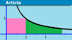
What’s the quantity on the proper such that the pink and inexperienced areas are equal?

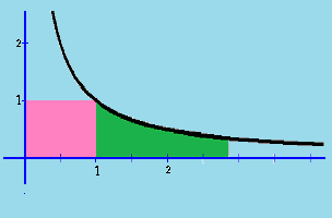
That is in trendy phrases the query
$$
1=int_1^x dfrac{1}{t},dt
$$
The answer is ##x=mathbf{e}=2.71828182845904523536028747135…## though it wanted the works of Isaac Newton (1643-1727) and Leonhard Euler (1707-1783) to acknowledge it. They discovered what we name the pure logarithm. It’s the integral of the hyperbola
$$
int dfrac{1}{x},dx = log_mathbf{,e} x = ln x
$$
Euler dealt loads with continued fractions. We checklist among the astonishing expressions which – simply perhaps – clarify Napier’s and Bürgi’s instinct.
start{align*}
mathbf{e}&=displaystyle 1+{frac {1}{1}}+{frac {1}{1cdot 2}}+{frac {1}{1cdot 2cdot 3}}+{frac {1}{1cdot 2cdot 3cdot 4}}+dotsb =sum _{ok=0}^{infty }{frac {1}{ok!}}
&=lim_{nto infty }dfrac{n}{sqrt[n]{n!}}=lim_{n to infty}left(sqrt[n]{n}proper)^{pi(n)}
&=2+dfrac{1mid}{mid 1}+dfrac{1mid}{mid 2}+dfrac{2mid}{mid 3}+dfrac{3mid}{mid 4}+dfrac{4mid}{mid 5}+dfrac{5mid}{mid 6}+ldots
&=3+dfrac{-1mid}{mid 4}+dfrac{-2mid}{mid 5}+dfrac{-3mid}{mid 6}+dfrac{-4mid}{mid 7}+dfrac{-5mid}{mid 8}+ldots
&=lim_{n to infty}left(1+dfrac{1}{n}proper)^n=lim_{stackrel{t to infty}{tin mathbb{R}}}left(1+dfrac{1}{t}proper)^t
left(1+dfrac{1}{n}proper)^n&<mathbf{e}<left(1+dfrac{1}{n}proper)^{n+1}
dfrac{1}{e-2}&=1+dfrac{1mid}{mid 2}+dfrac{2mid}{mid 3}+dfrac{3mid}{mid 4}+dfrac{4mid}{mid 4}+ldots
dfrac{e+1}{e-1}&=2+dfrac{1mid}{mid 6}+dfrac{1mid}{mid 10}+dfrac{1mid}{mid 14}+ldots
finish{align*}
Jakob Steiner (1796-1863) has proven in 1850 that ##mathbf{e}## is the uniquely outlined optimistic, actual quantity that yields the best quantity by taking the foundation with itself, a worldwide most:
$$
mathbf{e}longleftarrow maxleft{f(x), : ,x longmapsto sqrt[x]{x},|,x>0right}
$$
Thus ##mathbf{e}^x > x^mathbf{e},(xneq mathbf{e}),## or by way of complexity principle: The exponential perform grows quicker than any polynomial.

If we have a look at that perform
$$
exp, : ,xlongmapsto mathbf{e}^x = sum_{ok=0}^infty dfrac{x^ok}{ok!}
$$
then we observe that
$$
D_x(exp) = D_xleft(sum_{ok=0}^infty dfrac{x^ok}{ok!}proper)=
sum_{ok=1}^infty kcdotdfrac{x^{k-1}}{ok!}=sum_{ok=0}^infty dfrac{x^ok}{ok!}
$$
and
$$
D_x(exp)=exp(x)=int exp(x),dx
$$

The ##mathbf{e}-##perform is a hard and fast level for differentiation and integration.

We have now good mounted level theorems for compact operators (Juliusz Schauder, 1899-1943), compact units (Luitzen Egbertus Jan Brouwer, 1881-1966), or Lipschitz steady features (Stefan Banach, 1892-1945). The latter is the anchor of one of the essential theorems about differential equations, the theorem of Picard-Lindelöf:
The preliminary worth downside
$$
start{instances}
y'(t) &=f(t,y(t))
y(t_0) &=y_0
finish{instances}
$$
with a steady, and within the second argument Lipschitz steady perform ##f## on appropriate actual intervals has a singular answer.

One defines a useful ##phi, : ,varphi longmapsto left{tlongmapsto y_0+int_{t_0}^t f(tau,varphi(tau)),dtauright}## for the proof and reveals, that ##y(t)## is a hard and fast level of ##phi## if and provided that ##y(t)## solves the preliminary worth downside.

Progress and the ##mathbf{e}-##perform

Let ##y(t)## be the dimensions of a inhabitants at time ##t##. If the relative development charge of the inhabitants per unit time is denoted by ##c = c(t,y),## then ##y’/y= c##; i.e.,

$$y’= cy$$

and so

$$y=mathbf{e}^{cx}.$$

Therefore the ##mathbf{e}-##perform describes unrestricted development. Nonetheless, in any ecological system, the sources out there to help life are restricted, and this in flip locations a restrict on the dimensions of the inhabitants that may survive within the system. The quantity ##N## denoting the dimensions of the biggest inhabitants that may be supported by the system is known as the carrying capability of the ecosystem and ##c=c(t,y,N).## An instance is the logistic equation
$$
y’=(N-ay)cdot yquad (N,a>0).
$$
The logistic equation was first thought of by Pierre-François Verhulst (1804-1849) as a demographic mathematical mannequin. The equation is an instance of how complicated, chaotic habits can come up from easy nonlinear equations. It additionally describes a inhabitants of dwelling beings, equivalent to a really perfect bacterial inhabitants rising on a bacterial medium of restricted dimension. One other instance is (roughly) the unfold of an infectious illness adopted by everlasting immunity, leaving a reducing variety of people vulnerable to the an infection over time. The logistic perform can be used within the SIR mannequin of mathematical epidemiology. Beside the stationary options ##yequiv 0## and ##yequiv N/a,## it has the answer
$$
y_a (t)= dfrac{N}{a}cdot dfrac{1}{1+kcdot mathbf{e}^{-Nt}}
$$
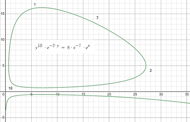
Populations are definitely extra complicated than even a restricted development if we think about predators and prey, say rabbits and foxes. The extra foxes there are, the less the rabbits, which results in fewer foxes, and the rabbit inhabitants can get better. The extra rabbits, the extra foxes will survive. This is called the pork cycle in financial science. The mannequin goes again to the American biophysicist Alfred J. Lotka (1880-1949) and the Italian mathematician Vito Volterra (1860-1940). The scale of the predator inhabitants will likely be denoted by ##y(t),## that of the prey by ##x(t).## The system of differential equations
$$
x'(t)= ax(t)-bx(t)y(t) ; , ;y'(t)= -cy(t)+dx(t)y(t)
$$
is known as Lotka-Volterra system. E.g. let ##a=10,b=2,c=7,d=1.## Then we get the answer ##y(t)^{10}mathbf{e}^{-2y(t)}=mathbf{e}^ok x(t)^{-7}mathbf{e}^{x(t)}.##

The Exponential Ansatz

We now have a look at the simplest differential equations and their options, linear strange ones over complicated numbers
$$
y’=Ayquadtext{ with a posh sq. matrix }A=(a_{ij})in mathbb{M}(n,mathbb{C})
$$
A posh perform
$$
y(t)=ccdot mathbf{e}^{lambda t}
$$
is an answer of this equation if and provided that ##lambda ## is an eigenvalue of the matrix ##A## and ##c## is a corresponding eigenvector. If ##A## has ##n## linearly impartial eigenvectors (that is the case, for instance, if A has ##n## distinct eigenvalues), then the system obtained on this method is a elementary system of options.

The concept holds in the actual case, too, however one has to cope with the actual fact, that some eigenvalues won’t be actual, and sophisticated options are often not those we’re serious about over actual numbers. The actual model of the theory has to cope with these instances and is thus a bit extra technical.

Let’s think about the Jordan regular type of a matrix. Then ##y’=Jy## turns into
$$
start{instances}
y_1’&=lambda y_1+y_2 y_2’&=lambda y_2+y_3
vdots &vdotsquad vdots
y_{n-1}’&=lambda y_{n-1}+y_n
y_n’&=lambda y_n
finish{instances}
$$
This technique can simply be solved by a backward substitution
$$
Y(t)=start{bmatrix}
mathbf{e}^{lambda t}&tmathbf{e}^{lambda t}&frac{1}{2}t^2mathbf{e}^{lambda t}&cdots&frac{1}{(n-1)!}t^{n-1}mathbf{e}^{lambda t}
0&mathbf{e}^{lambda t}&tmathbf{e}^{lambda t}&cdots&frac{1}{(n-2)!}t^{n-2}mathbf{e}^{lambda t}
0&0&mathbf{e}^{lambda t}&cdots&frac{1}{(n-3)!}t^{n-3}mathbf{e}^{lambda t}
vdots&vdots&vdots&ddots&vdots
0&0&0&cdots&mathbf{e}^{lambda t}
finish{bmatrix}
$$
The collection
$$
mathbf{e}^{B}=I+B+dfrac{B^2}{2!}+dfrac{B^3}{3!}+ldots
$$
converges completely for all ##B## so we get
$$
left(mathbf{e}^{At}proper)’=Acdot mathbf{e}^{At}
$$
and located a elementary matrix for our differential equation system, particularly
$$
Y(t)=mathbf{e}^{At}quad textual content{with}quad Y(0)=I
$$

An essential generalization in physics is periodic features. Say we’ve got a harmonic, ##omega ##-periodic system with a steady ##A(t)##
$$
x'(t)=A(t)x(t)quadtext{with}quad A(t+omega )=A(t)
$$
For it’s elementary matrix ##X(t)## with ##X(0)=I## holds
$$
X(t+omega )=X(t)Cquadtext{with a non-singular matrix}quad C=X(omega )
$$
##C## may be written as ##mathbf{e}^{omega B}## though the matrix ##B## isn’t uniquely decided due to the complicated periodicity of the exponential perform.

Theorem of Gaston Floquet (1847-1920)

##X(t)## with ##X(0)=I## has a Floquet illustration
$$
X(t)=Q(t)mathbf{e}^{ B t}
$$
the place ##Q(t)in mathcal{C}^1(mathbb{R})## is ##omega##-periodic and non-singular for all ##t.##

Allow us to lastly think about a extra subtle, however essential instance: Lie teams. They happen as symmetry teams of differential equations in physics. A Lie group is an analytical manifold and an algebraic group. Its tangent area on the ##I##-component is its corresponding Lie algebra. The latter will also be analytically launched as left-invariant (or right-invariant) vector fields. The connection between the 2 is straightforward: differentiate on the manifold (Lie group) and also you get to the tangent area (Lie algebra), combine alongside the vector fields (Lie algebra), and also you get to the manifold (Lie group).

The Lie By-product

“Let ##X## be a vector discipline on a manifold ##M##. We are sometimes serious about how sure geometric objects on ##M##, equivalent to features, differential types and different vector fields, range underneath the circulate ##exp(varepsilon X)## induced by ##X##. The Lie spinoff of such an object will in impact inform us its infinitesimal change when acted on by the circulate. … Extra usually, let ##sigma## be a differential type or vector discipline outlined over ##M##. Given some extent ##pin M##, after ‘time’ ##varepsilon## it has moved to
##exp(varepsilon X)## with its unique worth at ##p##. Nonetheless, ##left. sigma proper|_{exp(varepsilon X)p}## and ##left. sigma proper|_p ##, as they stand are, strictly talking, incomparable as they belong to totally different vector areas, e.g. ##left. TM proper|_{exp(varepsilon X)p}## and ##left. TM proper|_p## within the case of a vector discipline. To impact any comparability, we have to ‘transport’ ##left. sigma proper|_{exp(varepsilon X)p}## again to ##p## in some pure manner, after which make our comparability. For vector fields, this pure transport is the inverse differential
start{equation*}
phi^*_varepsilon equiv d exp(-varepsilon X) : left. TM proper|_{exp(varepsilon X)p} rightarrow left. TM proper|_p
finish{equation*}
whereas for differential types we use the pullback map
start{equation*}
phi^*_varepsilon equiv exp(varepsilon X)^* : wedge^ok left. T^*M proper|_{exp(varepsilon X)p} rightarrow wedge^ok left. T^*M proper|_p
finish{equation*}
This enables us to make the overall definition of a Lie spinoff.” [Olver]

The exponential perform comes into play right here, as a result of the exponential map is the pure perform that transports objects of the Lie algebra ##mathfrak{g}## to these on the manifold ##G##, a type of integration. It’s the identical cause we used the exponential Ansatz above since differential equations are statements about vector fields. If two matrices ##A,B## commute, then we’ve got
$$
textual content{addition within the Lie algebra }longleftarrow mathbf{e}^{A+B}=mathbf{e}^{A}cdot mathbf{e}^{B}longrightarrow
textual content{ multiplication within the Lie group}
$$
The standard case of non-commuting matrices is much more sophisticated, nonetheless, the precept stands, the conversion of multiplication to addition and vice versa. E.g., circumstances of the multiplicative determinant (##det U = 1##) for the (unitary) Lie group turns right into a situation of the additive hint (##operatorname{tr}S=0##) for the (skew-Hermitian) Lie algebra.

The Lie spinoff alongside a vector discipline ##X## of a vector discipline or differential type ##omega## at some extent ##p in M## is given by
start{equation*}
start{aligned}
mathcal{L}_X(omega)_p &= X(omega)|_p &= lim_{t to 0} frac{1}{t} left( phi^*_t (left. omega proper|_{exp(t X)_p})- omega|_p proper)
&= left. frac{d}{dt} proper|_{t=0}, phi^*_t (left. omega proper|_{exp(t X)_p})
finish{aligned}
finish{equation*}
On this type, it’s apparent that the Lie spinoff is a directional spinoff and one other type of the equation we began with.

Each, Lie teams and Lie algebras have a so-called adjoint illustration denoted by ##operatorname{Advert}, , ,mathfrak{advert},## resp. Inside automorphisms (conjugation) on the group degree grow to be inside derivations (linear maps that obey the Leibniz rule usually, and the Jacobi identification specifically) on the Lie algebra degree. Let ##iota_y## denote the group conjugation ##xlongmapsto yxy^{-1}.## Then the spinoff on the level ##I## is the adjoint illustration of the Lie group (on its Lie algebra as illustration area)
$$
D_I(iota_y)=operatorname{Advert}(y), : ,Xlongmapsto yXy^{-1}
$$
The adjoint illustration ##mathfrak{advert}## of the Lie algebra on itself as illustration area is the left-multiplication ##(mathfrak{advert}(X))(Y)=[X,Y].## Each are associated by
$$
operatorname{Advert}(mathbf{e}^A) = mathbf{e}^{mathfrak{advert} A}
$$

Sources